Computer lab 2: Sequencing quality control

This computer lab picks up as the sequencing machine has finished. Even if the sequencing machine did run ok there is no guarantee that the data is actually what we expect and the quality is good enough to use in our downstream analysis.

As the sequencing machine finishes it usually outputs some QC report, for Illumina machines this is in binary file that can be opened with the Sequencing Analysis Viewer (SAV) but could also be a text file or similar. This QC-report usually contains information on how the sequencing went, i.e. how much data were produced, clustering and average basequality etc. If several samples were pooled there is also information on how much data each index(-pair) got, and how much of the data actually contains the specified indexes.

Prerequisites

IGV
Web browser
Access to Uppmax project (uppmax2024-2-1)

If running locally:

Singularity (not available on Mac M1 silicon chip and above)
awk

Files

Can be found at the Uppmax project (uppmax2024-2-1). To ensure that you don't accidentally overwrite someone elses file start by copying the entire lab2_qc folder to your home (or local computer). Either download the entire folder locally or all work can be done in your own homefolder on Pelle.

mkdir ~/${course_folder}
cp -r /proj/uppmax2024-2-1/nobackup/lab_files/lab2_qc ~/${course_folder}
cd ~/${course_folder}/lab2_qc/

Common Quality Values

While running a bioinformatic pipeline it is important to continuously collect QC-values, this ensures that each step work as expected and can help you identify where and what happened if something gives unexpected results or crashes.

qcvalues dag

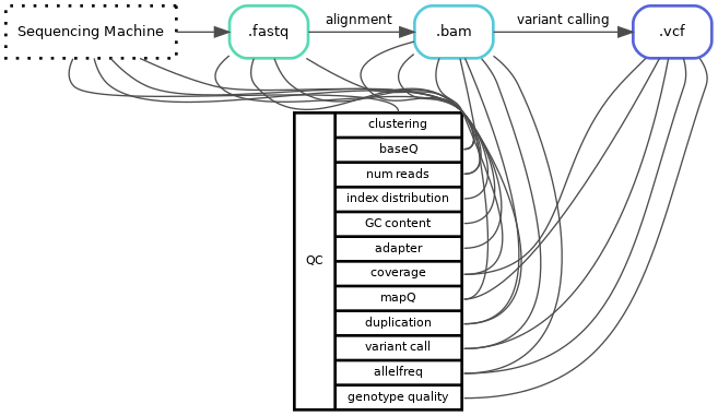
One issue or hurdle is that the same word can be used for different quality-values, it can also be the same value but calculated at different timepoints or the algorithm might differ depending on which program you use. For example duplication rate is a value of how many copies of the same read your library has, this can be estimated optically from the fastq-files or calculated after the reads have been aligned to your reference genome. Even if you calculate the duplication rate on the same file the algorithm can also differ between different programs (or even version of program). For example, how you define a duplicated read can differ, do you look at just the starting point or do you look at both the starting and end position of the reads. Therefore, it is always important to know how and on what file a value is calculated.

Another important factor to keep in mind is what kind of library you are looking at, capture, amplicon, pcr-free or even long-read all differs in expected values and results, and the values are often not comparable across methods.

Sequencing methods

Short Read Sequencing: most common sequencing method, read length ~50-150 bp.
Long Read Sequencing: allows for detection of complex SVs, read length ~5000-30000 bp.

PCR-free: sequencing library created without the use of PCR amplification.
(Hybridization) Capture: target sequencing using baits to "fish out" regions of interest.
Amplicon: target sequencing using primers to amplify specific targets.

Number of reads

Number of reads are what they sound like, how many reads do you have in your sample file(s). Often this variable is used to check if the sequence machine and pooling behaved as expected. This number is also used to calculate pooling, or expected output if you change flowcell/sequencing machine size.

Number of reads are calculated either directly in the sequencing machine, raw fastq or even the aligned bamfiles.

Question 1

If you get a lower number of reads for a sample than expected, what could be the cause of this? List possible wet lab errors, input file errors, sequencing machine errors, and/or analysis errors.

Example of programs that calculate Number of Reads:

SAV/sequence machine run stats
FastQC
Samtools stats
Picard HSMetrics

Question 2

Explain why the parameter "Number of Reads" within SampleA and B differ between different programs for this Illumina Nextseq run.

Sample	FastQC: `Total Sequences`	Samtools stats: `raw total sequences`	Picard HSMetrics: `TOTAL_READS`
SampleA	5M	8M	10M
SampleB	5.3M	9.2M	11M

Tip

Commands used to produce QC output:
FastQC: fastqc --quiet --outdir qc/fastqc/ fastq/sampleA_R1_001.fastq.gz
Samtools stats: samtools stats -t design_file.bed alignment/sampleA.bam > qc/samtools_stats/sampleA.samtools_stats.txt
Picard HsMetrics: gatk CollectHsMetrics -COVERAGE_CAP 500 -BAIT_INTERVALS design_file.intervals -TARGET_INTERVALS design_file.intervals -INPUT alignment/sampleA.bam -OUTPUT qc/picard_collect_hs_metrics/sampleA.HsMetrics.txt

Percent [%] mapped

After trimming away low quality reads and bases, the reads are aligned to a reference genome. The percent of reads that are mapped is often tracked during this step. This is to measure how well your data match the genome reference provided. This value is usually provided as a QC value from the alignment software you have used, e.g. bwa or minimap2 or any QC-checks done on aligned files.

Coverage

A measurement of how well covered your sample is. Usually defined as "Y" X coverage, where for example 40X coverage is normal in whole genome sequencing (WGS). This means that the average position is covered by Y number of reads. There are many different programs that calculate coverage (often in combination with other QC parameters), some examples are:

Question 3

Calculate the average coverage of TP53's exon3 (hg19: chr17:7579312-7579590) in SampleB with mosdepth.
Either you do this locally on your computer (need to have singularity available), or on Uppmax.
(Bam-file aligned to Hg19 reference genome.)

cd ~/${course_folder}/lab2_qc/
module load mosdepth/0.3.12
mosdepth sampleB-output ${path_to_file}/sampleB_subset.bam

If you are running locally, you need to download the bamfile and index files from Uppmax first, and then run it.

# Files needed: sampleB_subset.bam and sampleB_subset.bam.bai
singularity exec docker://hydragenetics/mosdepth:0.3.2 mosdepth sampleB-output sampleB_subset.bam

Tip

Looking into mosdepth documentation or using the built-in help mosdepth --help, is there a parameter that can help you restrict your calculation to only the region of interest?

Tip

How would you translate the region into a bedfile format?
chrA X Y
To get the coordinates into a file you can use echo:
echo -e "chrA\tX\tY" > design.bed
The -e will ensure that echo translates the \t to a tab.

Coverage distribution

Coverage distribution describes how the aligned reads are divided over the reference genome. Are they isolated to certain areas? Are some areas not covered properly? Are all regions covered the same?
Just like you did in lab 1, you can identify sequencing method by just looking at the distribution i.e. in the coverage track in IGV. In-depth coverage distribution is also used to estimate CNVs by most CNV-algorithms.

mosdepth_percontig

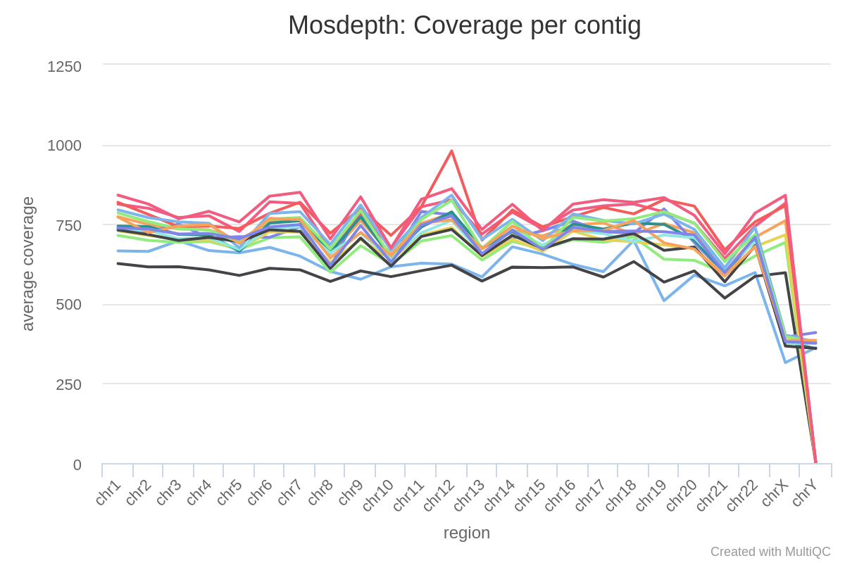
Question 4

Looking at the coverage distribution (above) for 16 samples (same capture panel, same sequence run), what stands out?

Tip

Look at the autosomal and the sex chromosomes separately.

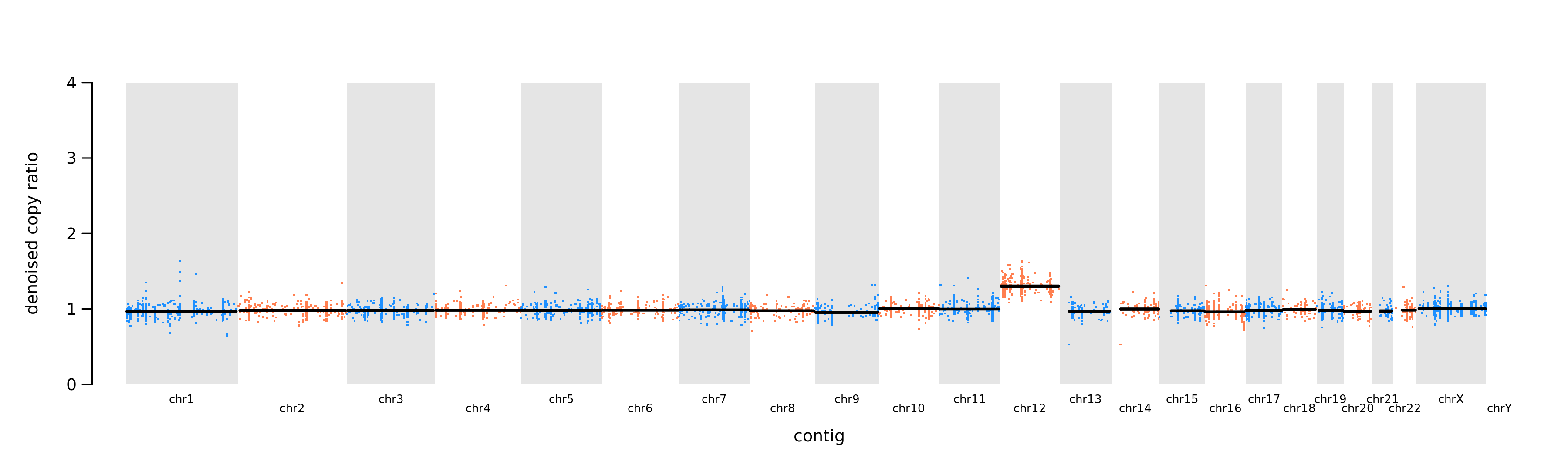
Autosomal chromosomes

Looking at the autosomal chromosome there is one sample that stands out. This is its normalised read counts (denoised copy ratio) plotted per chromosome. What does that tell us?
cnv_profile

Sex chromosomes

How many copies do we have of the sex chromosomes compared to autosomal, and how does this correlate to coverage?

Fold80

A more quantitative value based on coverage distribution is the fold 80 base penalty value calculated by e.g. Picard CollectHsMetrics. The Fold80 is defined as the fold change of non-zero read coverage needed to bring 80% of the ROI bases to the observed mean coverage, or a bit simpler put: how much more sequencing is required to bring 80% of the target bases to the mean coverage. So for a fold80 of 1.3 (which is a good value) 30% extra reads would be enough to bring 80% of the targets bases up to mean coverage.

Coverage breadth

Yet another common measurement of coverage is coverage breadth, or % ≥ Yx as it is often described as. This means that X % of the genome or target regions is covered by at least Y reads. By default several of these levels are calculated in most of the Picard metrics programs (depending one your sequencing method which collect metrics you run may vary). Since this is such a popular value many coverage programs often calculates breadth and allows you to specify your own specific thresholds if needed. The most common program used are the Picard metrics algorithms. Since this is a measurement of coverage over a given target it is important to keep track of what region/target this is calculated over to be able to compare numbers.

Why might the coverage breadth vary for the same human WGS (reference genome HG38) sample (same fastq files used) calculated with different pipelines? Discuss using the following keywords: target, qc-program, read filtering.

Name	PipelineA: Median Cov	PipelineA: % ≥ 30x	PipelineB: Median Cov	PipelineB: % ≥ 30x
SampleC	34	91	34	99

Duplication rate

The duplication rate is the fraction of mapped reads marked as duplicate reads in a particular data set. In contrast to overlapping reads, duplicate reads offer no additional information and are removed from sequencing data during the bioinformatic pipeline, a process known as deduplication. With other words duplicate reads are identical reads which are an artifact/bias introduced by a method; biological or technical (usually but not exclusively PCR), and will not give any new information and should therefore be flagged and remove from your dataset.

As for most QC-values, duplication rate can be calculated at many different stages and the definition can vary depending on algorithm.

The most common program for calculating the duplication rate on unaligned reads is FastQC. FastQC can either be a part of the bioinformatic pipelines or on some newer sequencing machines it is included in the "SAV".

For aligned reads, Picard MarkDuplicates is the most common program that identifies, flags and records outputs statistics of duplicates reads, but there are plenty of other programs and in-house solutions that does the same thing. Picard also has a program called Collect Duplicate Metrics which calculates the duplication rate on a previously duplication-marked bamfile.

Question 5

Use the files in lab2_qc/-folder answer the following questions:
Find the estimated duplication rate for sampleD from both FastQC and Picard CollectDuplicateMetrics. Fill in values in the table in question 6.

Tip

Checkout the output from the different programs under the qc-folder.

Explain why the duplication rate differs between FastQC and Picard MarkDuplicates/CollectDuplicateMetrics?

Tip

Check-out FastQC's documentation and compare it with Picard Markduplicate's.

Question 6

Fill out the table below with the missing values for sampleD.

Tip

Navigate the different outputs under the qc-folder to find the missing values for sampleD.

Programs

Number of reads: fastqc
Duplication rate: fastqc or collect duplicate metrics
Mean coverage: mosdepth
Fold80: Picard HsMetrics

Sample	Total sequences (M Seqs)	Duplication rate	Mean Coverage	Fold80
SampleD		FastQC: CollectDuplicateMetrics:

MultiQC

As you might have notice it takes quite a while to identify and find the different QC-values to track. To combat the never-ending file searching and enable easier tracking of QC-values the program MultiQC is often used. MultiQC aggregate the different QC-values into a single report. MultiQC only aggregate results from other programs (over 100 tools are automatically included, but you can also build your own tables or plots) and never does any calculation, therefore what values you can find and the layout of a MultiQC report varies a lot. It all depends on which programs you have run and input into MultiQC. MultiQC also allows you to configure almost all parts of the report with a config so a MultiQC-report does not always look like a "MultiQC-report".

The report is a self-contained interactive .html-file where you can adapt/configure/highlight etc the plots and tables directly in your web-browser. It also allows for an easy export of table and plots if needed.

Question 7

Open the provided MultiQC-report (lab2_qc/MultiQC_DNA_report.html) and "play around" with the different tools and parameters. Once you feel ready upload a screen-print of the MultiQC report with sampleP highlighted using the "Toolbox" on the right side of the report.

Question 8

Fill in the table below, as in Question 6, but for SampleE with the values found in the MultiQC report.

Tip

For all MultiQC tables you can configure and choose which columns to view by clicking the Configure Columns-button.

Sample	Total sequences (M Seqs)	Duplication rate	Mean Coverage	Fold80
SampleE		FastQC: CollectDuplicateMetrics:

Variant Quality

The next step after you have validated the quality of the sequence run is variants. How do we know that a variant we see is real and not an artifact?

BaseQ and MapQ

There are several different ways and steps to validate a variant. Most variant callers have build-in filtering steps that ensures that the variants reported are filtered or at least flagged if the confidence is low. One of the most basic way is to look at the base quality of the variant's alternative bases. However, the baseQ vary depending on sequencing machine and/or version of said machine. A good rule-of-thumb is that you always want a phred-score of at least 20 to be able to trust a base-call.

The other quality-value that is usually included are mapping quality, how well a read has aligned to exactly that specific region of the reference genome. Different aligners use different scoring algorithm and therefore it is hard to compare quality values across programs. For some more in-depth reading see here and here for example.

Question 9

Open .bam file called sampleD_subset.bam in IGV, and navigate to chr17:7577114. How many T calls have a base quality below Q20?

Tip

Sort the position based on base (right click -> sort by -> base). By default IGV only displays 100 reads. To show all reads click View -> PreferencesUnder view -> Preferences -> Alignments and un-tick "Downsampling reads". Also make sure that Shade mismatched bases by quality is checked.

Genotype Quality

Most variant callers have some sort of genotype quality scoring available for each variant call. The problem here is that it is not standardized and each caller can have completely different values making them hard to compare. For example for GATK produced vcf-files there are several different quality values, there is the QUAL column as well as the GQ and PL fields in the FORMAT column. For more in-depth info on the different vcf columns and annotation for GATK see more info here. While other programs might also call their quality value by the same name, their definition is often completely different.

gq_values

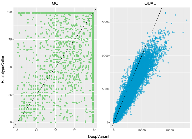
If we compare two variantcallers (GATK's Haplotypcaller and Google's Deepvariant); both specialized on germline calling, both use the flag GQ and the QUAL column as a quality measurements, we see a clear difference on both of the quality scores for the same variants. That said, the genotype quality score is not useless, but actually a good quality measurement of a variant call, you just always have to know how the file were produced and what scoring thresholds are considered "good" for that specific program.

Extra assigment

Coverage breadth

Finding coverage breadth is not always easy. In the mosdepth_bed folder, locate the qc/mosdepth_bed/sampleD_T.thresholds.bed.gz file and have a look inside it with less ${file} (use q to exit). In this file the number of bases covered per region is presented for a set of different threshold values.

Fill in the table for coverage breadth for sampleD. You want the total coverage breadth, not per region.

Sample	% ≥ 200x	% ≥ 500x
sampleD

To calculate the % ≥ Yx you need to add together coverage for the entire design and then divide it by the total length of the design: $$ \frac{\sum covered\ bases} {\sum region\ length} $$

For example:

chrom	start	end	10x
chrA	1	11	2
chrA	20	25	0

Would give us $$ \frac {(2+0)} {(11-1)+(25-20)}=0.1333... $$ i.e. 13.3 % ≥ 10x

Tip

Try piping the output from zcat (to open the gzipped file "on/the/fly") to awk to calculate the coverage breadth using the formula above.

Full command

Identify which columns you are interested in and use it to replace $x with the column number (1-index) in the script below:

zcat qc/mosdepth_bed/sampleD_T.thresholds.bed.gz | awk 'NR>1{tot_length+=$3-$2;tot_bases+=$x}END{print tot_bases"/"tot_length"="tot_bases/tot_length}'

Step-by-step explanation:

zcat allows for reading the gzipped file without extracting it.
awk is a handy string manipulating program
NR>1 means skip the first line since that line is the header.
tot_length+=$3-$2 is a cumulative variable that increases with the length of the region for each row. The values in column 2 is subtracted from column 3 and the sum is added to the variable tot_length.
tot_bases+=$x is the cumulative value of your desired column.
END just means do the following once the end of the file is reached.
print print the following to the command line.

Compare your values with the value found in MultiQC.

See if you can find a way of calculating the coverage breadth of 450x for chromosome 17 in sampleD_subsample. Use the file lab2_qc/chr17_hg19.bed to restrict the calculations to regions on chromosome 17.

Tip

Which program was used to produce the original file? Is there a way of change the input parameters to calculate different level of coverage breadth?

Background and artifacts

Another step for validating a variant is eliminating the risk that the variant actually is a sequencing artifact or just background from a "messy" region.

To identify artifacts you have to be able to separate the real variant calls from the variants that look like a real disease causing variant but is actually a call introduced by of some sort of bias. What further complicates the process is that since in sequencing we use organic enzymes and proteins we often introduce artifacts in the same region as the cell might have trouble processing the DNA, such as long repetitive sequences or homopolymers. Some artifacts are easier to identify than others, for example sequencing chemistry can affect our ability to sequence certain areas.

What is the most classic artifact introduced by 2-color chemistry in the Illumina sequencing?

To identify background noise you need to separate an actual call to the normal noise or distribution of basecalls. No technique has 100 % base recall, and even if that was the case we still primarily sequence short-read today, there is always a chance that your read actually originates from somewhere else. Most background is below 5 % allele frequency otherwise it moves towards being an artifact, so for most high frequency variants we are safe. The problem arises when we want to be able to detect low frequency variants. To be able to detect low frequency variants we have to sequence deeper and have greater prior knowledge of the methods.

Both background and artifacts is a lot easier identify if a normal pool of samples is available to compare your data with. A normal pool consists of a number (the more the better) of "healthy" samples processed identical (or as close as possible) as your sample. Small and big biases are always introduced what ever we do, therefore it is important to spread out the normal samples in several batches to mitigate batch-bias. And different sequencing machines use different chemistry you need a normal-pool for each machine type you plan to include.